Raster calculation

calc() evaluates an R expression for each pixel in a raster layer or stack of layers. Each layer is defined by a raster filename or dataset object, band number, and a variable name to use in the R expression. If not specified, band defaults to 1 for each input raster. Variable names default to LETTERS if not specified (A (layer 1), B (layer 2), ...). All of the input layers must have the same extent and cell size. The projection will be read from the first raster in the list of inputs. Individual pixel coordinates are also available as variables in the R expression, as either x/y in the raster projected coordinate system or inverse projected longitude/latitude. Multi-band output is supported as of gdalraster 1.11.0.

Usage

calc(
  expr,
  rasterfiles,
  bands = NULL,
  var.names = NULL,
  dstfile = tempfile("rastcalc", fileext = ".tif"),
  fmt = NULL,
  dtName = "Int16",
  out_band = 1L,
  options = NULL,
  nodata_value = NULL,
  setRasterNodataValue = FALSE,
  write_mode = "safe",
  quiet = FALSE,
  return_obj = FALSE,
  ...
)

Arguments

expr

An R expression as a character string (e.g., "A + B").

rasterfiles

Input rasters, either a character vector of filenames, or a list with each element either a filename as character string or an object of class GDALRaster (must be an open dataset for the latter).

bands

Integer vector of band numbers to use for each raster layer.

var.names

Character vector of variable names to use for each raster layer.

dstfile

Either a character string with the output raster filename, or an object of class GDALRaster with which to write output. If given as an object, the dataset must be open for write access, and the arguments below related to raster creation are ignored (i.e., fmt, dtName, options, setRasterNodataValue). The write_mode must be set to "update" for writing with an existing dataset object.

fmt

Output raster format name (e.g., "GTiff" or "HFA"). Will attempt to guess from the output filename if not specified.

dtName

Character name of output data type (e.g., Byte, Int16, UInt16, Int32, UInt32, Float32).

out_band

Integer band number(s) in dstfile for writing output. Defaults to 1L. Multi-band output is supported as of gdalraster 1.11.0, in which case out_band would be a vector of band numbers.

options

Optional list of format-specific creation options in a vector of "NAME=VALUE" pairs (e.g., options = c("TILED=YES", "COMPRESS=LZW") to set LZW compression during creation of a tiled GTiff file).

nodata_value

Numeric value to assign if expr returns NA.

setRasterNodataValue

Logical value. TRUE will attempt to set the raster format nodata value to nodata_value, or FALSE not to set a raster nodata value on the output dataset.

write_mode

Character string. Name of the file write mode for output. One of:

safe - execution stops if dstfile already exists (no output written)
overwrite - if dstfile exists it will be overwritten with a new file
update - if dstfile exists, will attempt to open in update mode, or write to the existing dataset if dstfile is given as an object

quiet

Logical value. If TRUE, a progress bar and informational messages will not be displayed. Defaults to FALSE.

return_obj

Logical value. If TRUE, an object of class GDALRaster opened on the newly created dataset will be returned. The default is FALSE.

...

Additional arguments, none currently supported.

Value

By default, returns the output filename invisibly. An object of class GDALRaster open on the output dataset will be returned if return_obj = TRUE.

Details

The variables in expr are vectors of length raster xsize (i.e., row vectors of the input raster layer(s), with length the number of raster columns). The expression should return a vector also of length raster xsize (an output row). Four special variable names are available in expr: pixelX and pixelY provide pixel center coordinates in projection units. pixelLon and pixelLat can also be used, in which case the pixel x/y coordinates will be inverse projected to longitude/latitude (in the same geographic coordinate system used by the input projection, which is read from the first input raster). Note that inverse projection adds computation time.

To refer to specific bands in a multi-band input file, repeat the filename or dataset object in rasterfiles and specify corresponding band numbers in bands, along with optional variable names in var.names, e.g.,


rasterfiles = c("multiband.tif", "multiband.tif")
bands = c(4, 5)
var.names = c("B4", "B5")

Output will be written to dstfile. To update a file that already exists, set write_mode = "update" and set out_band to an existing band number(s) in dstfile (new bands cannot be created in dstfile). dstfile can optionally be given as an object of class GDALRaster open for write access.

To write multi-band output, expr must return a vector of values interleaved by band. This is equivalent to, and can also be returned as, a matrix m with nrow(m) equal to length() of an input vector, and ncol(m) equal to the number of output bands. In matrix form, each column contains a vector of output values for a band. length(m) must be equal to the length() of an input vector multiplied by length(out_band). The dimensions described above are assumed and not read from the return value of expr.

Examples

## Using pixel longitude/latitude

# Hopkins bioclimatic index (HI) as described in:
# Bechtold, 2004, West. J. Appl. For. 19(4):245-251.
# Integrates elevation, latitude and longitude into an index of the
# phenological occurrence of springtime. Here it is relativized to
# mean values for an eight-state region in the western US.
# Positive HI means spring is delayed by that number of days relative
# to the reference position, while negative values indicate spring is
# advanced. The original equation had elevation units as feet, so
# converting m to ft in `expr`.

elev_file <- system.file("extdata/storml_elev.tif", package="gdalraster")

# expression to calculate HI
expr <- "round( ((ELEV_M * 3.281 - 5449) / 100) +
                ((pixelLat - 42.16) * 4) +
                ((-116.39 - pixelLon) * 1.25) )"

# calc() writes to a tempfile by default
hi_file <- calc(expr = expr,
                rasterfiles = elev_file,
                var.names = "ELEV_M",
                dtName = "Int16",
                nodata_value = -32767,
                setRasterNodataValue = TRUE)
#> calculating from 1 input raster...
#> ================================================================================
#> output written to /tmp/RtmphHzZRN/rastcalc228975750b75.tif

ds <- new(GDALRaster, hi_file)
# min, max, mean, sd
ds$getStatistics(band = 1, approx_ok = FALSE, force = TRUE)
#> 0...10...20...30...40...50...60...70...80...90...100 - done.
#> [1] 37.000000 57.000000 44.928763  4.384622
ds$close()

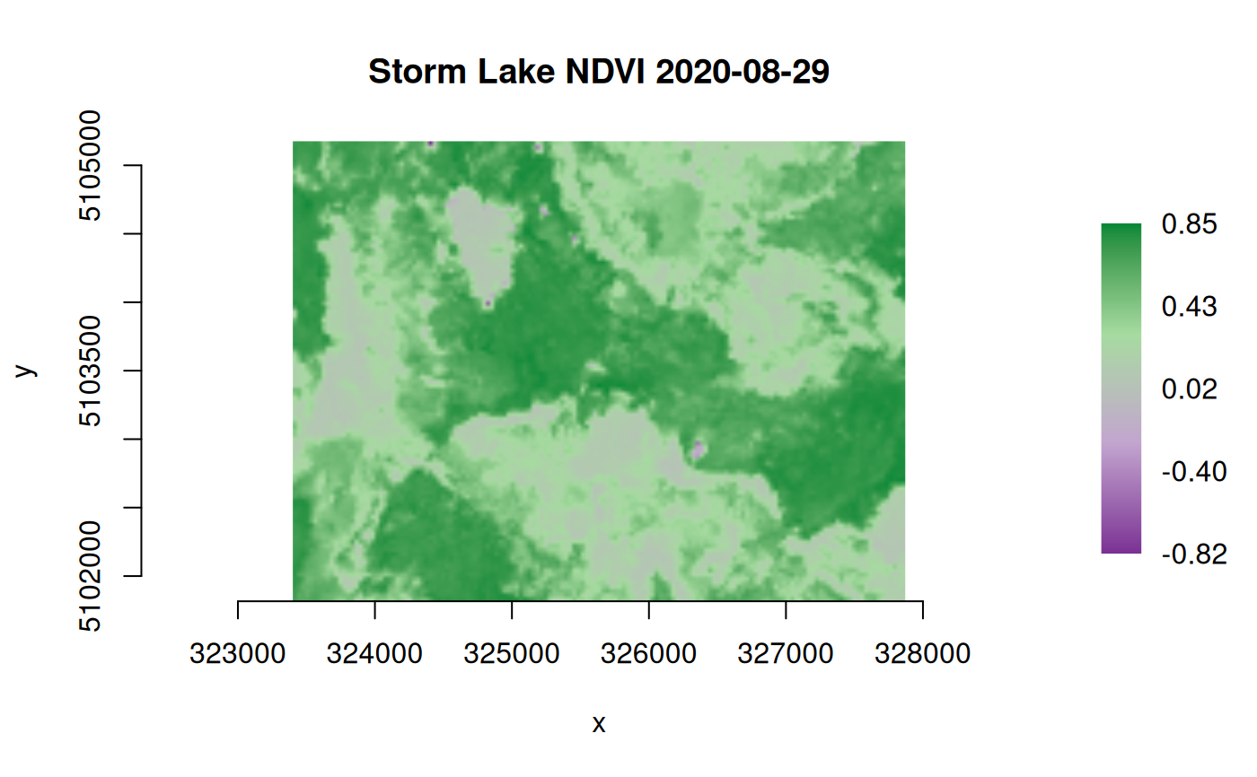
## Calculate normalized difference vegetation index (NDVI)
## input rasters given as dataset objects
## output to an in-memory raster (MEM format)

# Landast band 4 (red) and band 5 (near infrared):
b4_file <- system.file("extdata/sr_b4_20200829.tif", package="gdalraster")
b4 <- new(GDALRaster, b4_file)
b5_file <- system.file("extdata/sr_b5_20200829.tif", package="gdalraster")
b5 <- new(GDALRaster, b5_file)

expr <- "((B5 * 0.0000275 - 0.2) - (B4 * 0.0000275 - 0.2)) /
         ((B5 * 0.0000275 - 0.2) + (B4 * 0.0000275 - 0.2))"

(ndvi <- calc(expr, list(b4, b5), var.names = c("B4", "B5"), fmt = "MEM",
              dtName = "Float32", setRasterNodataValue = TRUE,
              return_obj = TRUE))
#> calculating from 2 input rasters...
#> ================================================================================
#> output written to in-memory-raster
#> C++ object of class GDALRaster
#>  Driver : In Memory Raster (MEM)
#>  DSN    : in-memory-raster
#>  Dim    : 149, 112, 1
#>  CRS    : NAD83 / UTM zone 12N (EPSG:26912)
#>  Res    : 30.000000, 30.000000
#>  Bbox   : 323400.853100, 5101815.783500, 327870.853100, 5105175.783500

plot_raster(ndvi, legend = TRUE,
            col_map_fn = c("#7b3294", "#c2a5cf", "#a6dba0", "#008837"),
            main = "Storm Lake NDVI 2020-08-29")


ndvi$close()
b4$close()
b5$close()

## Reclassify a variable by rule set

# Combine two raster layers and look for specific combinations. Then
# recode to a new value by rule set.
#
# Based on example in:
#   Stratton, R.D. 2009. Guidebook on LANDFIRE fuels data acquisition,
#   critique, modification, maintenance, and model calibration.
#   Gen. Tech. Rep. RMRS-GTR-220. U.S. Department of Agriculture,
#   Forest Service, Rocky Mountain Research Station. 54 p.
# Context: Refine national-scale fuels data to improve fire simulation
#   results in localized applications.
# Issue: Areas with steep slopes (40+ degrees) were mapped as
#   GR1 (101; short, sparse dry climate grass) and
#   GR2 (102; low load, dry climate grass) but were not carrying fire.
# Resolution: After viewing these areas in Google Earth,
#   NB9 (99; bare ground) was selected as the replacement fuel model.

# look for combinations of slope >= 40 and FBFM 101 or 102
lcp_file <- system.file("extdata/storm_lake.lcp", package="gdalraster")
rasterfiles <- c(lcp_file, lcp_file)
var.names <- c("SLP", "FBFM")
bands <- c(2, 4)
tbl <- combine(rasterfiles, var.names, bands)
#> combining 2 rasters...
#> 0...10...20...30...40...50...60...70...80...90...100 - done.
nrow(tbl)
#> [1] 449
tbl_subset <- subset(tbl, SLP >= 40 & FBFM %in% c(101,102))
print(tbl_subset)       # twelve combinations meet the criteria
#>     cmbid count SLP FBFM
#> 8     423     2  44  102
#> 10    421     1  49  102
#> 13    409    15  41  102
#> 37    365     1  44  101
#> 45    420     3  43  102
#> 93    283    17  40  101
#> 160   417     4  42  101
#> 225   397    11  42  102
#> 338   328    16  40  102
#> 346   338    10  41  101
#> 364   418     3  47  102
#> 408   341     2  43  101
sum(tbl_subset$count)   # 85 total pixels
#> [1] 85

# recode these pixels to 99 (bare ground)
# the LCP driver does not support in-place write so make a copy as GTiff
tif_file <- file.path(tempdir(), "storml_lndscp.tif")
createCopy("GTiff", tif_file, lcp_file)
#> 0...10...20...30...40...50...60...70...80...90...100 - done.
#> [1] TRUE

expr <- "ifelse( SLP >= 40 & FBFM %in% c(101,102), 99, FBFM)"
calc(expr = expr,
     rasterfiles = c(lcp_file, lcp_file),
     bands = c(2, 4),
     var.names = c("SLP", "FBFM"),
     dstfile = tif_file,
     out_band = 4,
     write_mode = "update")
#> calculating from 2 input rasters...
#> ================================================================================
#> output written to /tmp/RtmphHzZRN/storml_lndscp.tif

# verify the ouput
rasterfiles <- c(tif_file, tif_file)
tbl <- combine(rasterfiles, var.names, bands)
#> combining 2 rasters...
#> 0...10...20...30...40...50...60...70...80...90...100 - done.
tbl_subset <- subset(tbl, SLP >= 40 & FBFM %in% c(101,102))
print(tbl_subset)
#> [1] cmbid count SLP   FBFM 
#> <0 rows> (or 0-length row.names)
sum(tbl_subset$count)
#> [1] 0

# if LCP file format is needed:
# createCopy("LCP", "storml_edited.lcp", tif_file)

Usage

Arguments

Value

Details

See also

Examples